Download PDF

Introduction

Choosing the proper weighting factor is crucial to obtaining the best curve fit and therefore, obtaining the curve fit parameter values that make the curve fit model as close as possible to the measured data points. Weighting will affect the influence of the data points at each concentration and give more importance, or weight, to certain data points or a particular part of the curve.

Weighting is a reflection of modeling the errors in the data and has been developed to account for the difference in absolute error at the different data points describing the curve¹ . In 4 parameter (4P) and 5 parameter (5P) dose-response curve fits, the absolute error is generally larger at the top of the curve than at the bottom due to increasing variation between replicates as the concentration increases. Larger standard deviations for points at the top of the curve can dominate the curve fit and estimation of the curve parameters.

Choosing the proper weighting factor will allow you to adjust the curve to be a better fit around responses with the smallest variance and a looser fit around responses with the largest variance². It is important to understand how variation within the data set is distributed to choose and apply the correct weighting factor. If the variation distribution is not known, then various weighting functions can be assessed as described in this application note.

When to use weighting

Curve weighting and selection of the weighting factor should be done after the best curve fit has been evaluated during the method development or the method validation when sufficient amounts of data are available. In all curve fit models, X (generally the concentration) is an independent variable and Y (the response) is a dependant variable. For homoscedatic data, where the standard deviation is the same at all sample concentrations, the best fit is an unweighted fit where no weighting factor is applied. However, weighting becomes useful with heteroscedastic data, where the standard deviation increases with the sample concentration as shown in Figure 1³.

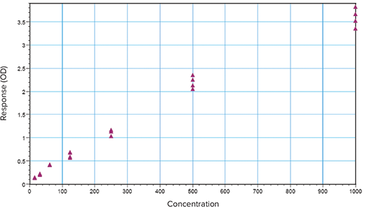
Figure 1. Heteroscedastic data. Scatter along the Y axis increases as the concentration increases.

Some curve fits, such as 4P and 5P curve fits, work to minimize the vertical errors between data points and the curve.

In doing so, the resulting curve fit may miss a number of the data points at lower concentrations as the curve is pulled upward from these points. This makes horizontal interpolation at these lower concentrations inaccurate. Weighting the curve with the correct factor will overcome this issue and lead to the most accurate estimate of the curve and therefore the most accurate concentration estimates from back calculated values.

Weighting factors

There are several weighting factors available to achieve precision and accuracy of curve fit parameters and estimated values. The most popular weighting involves adjusting the data by factors related to the inverse of the response³ : 1/Y² or 1/Y. 1/Y² is called relative weighting and is appropriate to use when you expect the average distance of the points from the curve to be higher when Y is higher, but the relative distance (distance/Y) to be a constant. 1/Y is called Poisson weighting and is useful when the errors in the Y values follows a Poisson distribution. This is the case when data scatter is due to counting error.

Other weighting methods involve adjusting the data by factors related to the inverse of the concentration: 1/X² or 1/X. These will weight points on the left part of the graph more than the right⁴ . The inverse of standard deviation weighting factor, 1/Std², allows more weight to be assigned to data points with low scatter. However, it should be used only when there are a number of replicates that reflect consistent differences in variability. The inverse of the sum of squares is used for variation that follows a Gaussian distribution or Turkey Biweight which reduces the influence of outliers. This and other weighting schemes will not be discussed here

How to use a weighting factor in SoftMax Pro 7

By default, SoftMax Pro^® 7 Software does not apply weighting to curve fits. This is referred to as Fixed Weight where the weighting factor is set to one for all data points of the curve fit. It also has the ability to apply a global fit or weight individual curves as shown in Figure 2

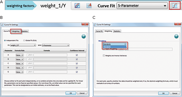
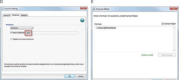
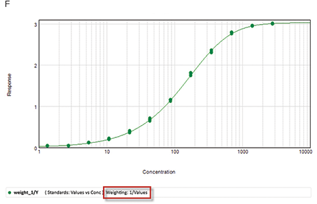
Figure 2. How to apply weighting in SoftMax Pro 7. (A) Select the Curve Fit Settings icon in the graph menu. (B) Select the weighting tab from the Curve Fit Settings window. (C) Choose the curve to be weighted by clicking on the drop down menu. Only the curves on the selected graph will appear. (D) Select “Apply Weighting”. Note that different curves that are on the same graph can be weighted independently. (E) Select the =f [x] formula icon and enter either a mathematical function such as 1/Values@Standards, where Values is the response at each concentration in the Standards group. (F) The weighting factor has been applied to the curve and should appear under the graph in the legend.

Measuring the goodness of a weighting factor in SoftMax Pro 7

As discussed in the previous application note, “Selecting the best curve fit in SoftMax Pro”, the goodness of the fit, and therefore the goodness of the applied weight on the curve fit, can be measured using the Sum of Squared Errors (SSE) and the Akaike’s Information Criterion (AIC) methods.

A protocol titled “Weighting factors tested in SoftMax Pro” has been developed and implemented with the necessary calculations so the most popular weighting factors: 1/Y, 1/Y² and 1/Std² can be tested and compared using the SSE and the AIC methods. This protocol is available for download on our protocol sharing website at www.softmaxpro.com. Figure 3 shows an example of homoscedastic data which should not require any weighting because there is very little scatter through the data set. Data were fitted to a 5P curve fit model and various weighting factors were applied: no weight (Figure 3A), 1/Y (Figure 3B), 1/Y² (Figure 3C), and 1/Std² (Figure 3D).

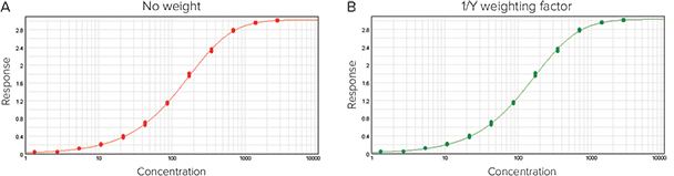
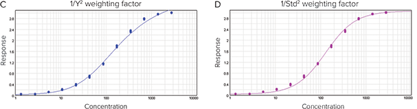
Figure 3. Weighting evaluation of homoscedastic data fitted to a 5P curve fit model where various weighting factors are applied: (A) no weight, (B) 1/Y, (C) 1/Y² and (D) 1/Std2. The scatter evaluation and the results are shown in Figure 4 and the residual plot of the data is represented in Figure 5.

Figure 4. Scatter evaluation of the homoscedastic data presented in Figure 3. (A) The graph shows constant standard deviation throughout the concentrations result report. (B) The R² value, SSE, AIC, and AICc. (C) The weighting results section from the protocol concludes that for both methods, no weight gives the best fit to the 5P curve.

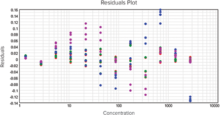
Figure 5. Residuals plot of the homoscedastic data presented in Figure 3. The residuals appear randomly scattered around zero indicating that the model describes the data well.

The next example illustrates the case of heteroscedastic data (Figures 6-8). Here the standard deviation increases as the response increases and generates a scatter (Figure 7A). Data were fit to a 5P curve fit model and various weighting factors were applied: no weight (Figure 6A), 1/Y (Figure 6B), 1/Y² (Figure 6C) and 1/Std² (Figure 6D). The results are summarized in Figure 7 and show that the 1/Y² weighting factor gave the best fit to the data set.

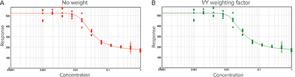
Figure 6. Weighting evaluation of heteroscedastic data fitted to a 5P curve fit model where various weighting factors are applied: (A) no weight, (B) 1/Y, (C) 1/Y² and (D) 1/Std². The scatter evaluation and the results are shown in Figure 7 and the residual plot of the data is represented in Figure 8.

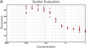
Figure 7. Scatter evaluation of the heteroscedastic presented in Figure 5. (A) The graph shows a scatter and variation within the data set. (B) The R² value, SSE, AIC, and AIC_c. (C) The weighting results section from the protocol concludes that for both methods, the weight of 1/Y² gave the best fit to the 5P curve.

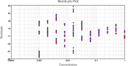
Figure 8. Residuals plot of the heteroscedastic data presented in Figure 6. The residuals do not appear randomly around zero, which indicates that the 5P model does not describe the data well regardless of the weighting applied.

Conclusion

A protocol has been developed with the SSE and the AIC methods to test the most common weighting factors with the curve fit model of choice within SoftMax Pro 7 Software. These statistical tests help to compare the goodness of the fit when different weighting factors are applied, allowing the most suitable weighting to be selected with confidence. However, it is imperative to ensure that a significant amount of data points are used to account for variation.

References

1. Gottschalk, P., Dunn, J. 2005. The 5-Parameter logistic: A characterisation and comparison with the 4-Parameter logistic, Analytical Biochemistry, 54-65.
2. Ledvij,M. 2003. Curve fitting made easy, The Industrial Physicist.
3. Dolan, J., 2009. Calibration Curves, PartV: Curve Weighting, LC.GC.
4. Kiser, M., and Dolan, j. 2004. Selecting the best curve fit, LC.GC Europe.

Learn more about SoftMax Pro Software >>

Download PDF